Replicate Analysis of Near-Infrared Western Blots

Introduction

Replicate measurements are critical for quantitative Western blot (QWB) analysis. The purpose of QWB is to monitor changes in the relative abundance or modification of a target protein within a group of samples. Does the experimental treatment cause an increase or decrease in target abundance, compared to the untreated or control condition?

Replicate samples confirm the validity of observed changes in protein levels. Without replication, it is impossible to know if an effect is real or simply an artifact of experimental noise or variation. Biological and technical replicates are both important, but each type of replicate addresses different questions (1, 2, 3).

Empiria Studio® Software lets you compare replicate samples on the same blot or across multiple blots. Go to licorbio.com/empiria to learn more.

Types of Replicate Measurements

Technical replicates are repeated measurements used to establish the variability of a protocol or assay, and determine if an experimental effect is large enough to be reliably distinguished from the assay noise (1).

Examples may include loading of multiple lanes with each sample on the same blot, running multiple blots in parallel, or repeating the blot with the same samples on different days.
Technical replicates evaluate the precision and reproducibility of an assay, to determine if the observed effect can be reliably measured. When technical replicates are highly variable, it is more difficult to separate the observed effect from the assay variation. You may need to identify and reduce sources of error in your protocol to increase the precision of your assay. Technical replicates do not address the biological relevance of the results.

Biological replicates are parallel measurements of biologically distinct and independently generated samples, used to control for biological variation and determine if the experimental effect is biologically relevant. The effect should be reproducibly observed in independent biological samples. Demonstration of a similar effect in another biological context or system can provide further confirmation.

Examples include analysis of samples from multiple mice rather than a single mouse, or from multiple batches of independently cultured and treated cells.
To demonstrate the same effect in a different experimental context, the experiment might be repeated in multiple cell lines, in related cell types or tissues, or with other biological systems.

An appropriate replication strategy should be developed for each experimental context. Several recent papers discuss considerations for choosing technical and biological replicates (1, 2, 3).

Reporting Changes in Relative Abundance

QWB methods typically use ratiometric analysis to determine relative abundance of the target protein and compare relative protein levels across a group of samples.

Ratiometric analysis is a form of "self-calibration" that expresses the relative abundance of target protein as a ratio between the experimental sample and the control. It compares the intensity of the target band in each experimental sample to the intensity of the target band in the control sample (4, 5, 6).

Normalize your QWB data using an appropriate internal loading control (such as total protein staining).
- Normalization mathematically corrects for small, unavoidable variations in sample loading and transfer by comparing the target protein to an internal loading control. More information is found in Quantitative Western Blot Normalization.
- See these resources to learn more about QWB normalization:
  
  Western Blot Normalization Handbook (licorbio.com/handbook)
  
  Western Blot Normalization: Challenges and Considerations White Paper (licorbio.com/normalizationreview)
Perform the ratiometric analysis, as described in Calculations for Replicate Analysis.
- The normalized signal intensity of the target band in each sample should be divided by the normalized intensity of the target band in the control sample.

The resulting ratios, expressed as fold change or percentage (%) change, are used to compare relative protein levels across the samples on your blot. Because all samples are compared to the control, these measurements are proportional and are independent of raw signal intensity.

Fold change is a unitless value that compares the relative abundance of a target protein to the control sample on the same membrane.

A value above 1.0 indicates an increase in abundance relative to the control; a value below 1.0 indicates decreased abundance (. Relative abundance of target protein, expressed as fold change and % change.).

Percentage (%) change is a unitless value similar to fold change that expresses changes in relative abundance as a percentage.

A positive percentage indicates increased abundance relative to the control; a negative percentage indicates decreased abundance (. Relative abundance of target protein, expressed as fold change and % change.).

**Table 2**. Relative abundance of target protein, expressed as fold change and % change.
Fold Change	% Change
1.0	0%
1.2	+20%
1.5	+50%
2.0	+100%
0.8	-20%
0.5	-50%
0.1	-90%

Keys to Success

Accurate QWB analysis requires a robust, well-characterized detection system. Data should be captured within the linear range of detection, with careful attention to limits of detection and saturation of strong bands. Methods should be sufficiently robust that the outcome is unaffected by trivial or unintended changes in the reagents and protocol (7‑8).

This protocol provides guidelines for characterizing the linear range of detection for your system: Determining the Linear Range for Quantitative Western Blot Detection (licorbio.com/LinearRange)
Relative changes in abundance can only be measured if they substantially exceed the variability of your measurement. See Data Interpretation, Data Interpretation, for guidelines.
Do not compare signal intensities between blots. Experimental variations in sample loading transfer conditions, antibody reagents, incubation times, and many other factors affect the raw signal intensities on each blot. Band intensity should only be analyzed by relative, ratiometric comparison to the control samples.
Every blot should include control samples (untreated, baseline, etc.) and be processed for detection with the same reagents, protocol, and imaging method. Fold change values can then be compared between blots loaded with the same control samples.

Experimental Design

Analysis of Replicate Samples on Separate Western Blots

Plan an appropriate strategy for technical and biological replicates in your experiment. It may be helpful to consult a statistician before you begin to generate data.
Collect replicate data that represent the desired experimental conditions (drug treatments, time course, dose-response, etc). A minimum of three replicates should be performed for each sample, including the controls.

Samples should be loaded in random order on each blot to minimize position effects. Sample placement on the blot (for example, in edge lanes vs. interior lanes) may affect signal intensity and introduce variability. Random sample placement will reduce the impact of position effects (4).

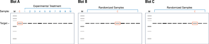
Figure 50. Replicate blot layout described in this protocol. Each gel is loaded with MW marker (M), control sample (C), and experimental samples (1-10). On blots B and C, control and experimental samples are loaded in random order.
Use this protocol to analyze and compare replicate samples on separate Western blots.
1. This protocol describes the analysis of three replicate blots (designated A, B, and C; see Figure 50), each loaded with a molecular weight marker, control sample, and 10 experimental samples.
2. This layout can be used to analyze either technical or biological replicates, depending on the nature of the samples you load. Appropriate interpretation of the resulting data will be specific to your samples and experimental context.
  - Technical replicates: Load the same group of control and experimental samples repeatedly, onto three (or more) separate gels, to generate replicate blots.
  - Biological replicates: Perform three (or more) independent experiments. Load each set of control and experimental samples onto its own separate gel, to generate replicate blots.

Quantitative Western Blot Normalization

Normalize your Western blot data, using an appropriate internal loading control.
1. Normalization mathematically corrects for small, unavoidable sample-to-sample and lane-to-lane variation by comparing the target protein to an internal loading control.
  
  Internal loading controls are endogenous reference protein(s) that are present in all samples at a stable level, and unaffected by the experimental conditions or treatments. The loading control serves as an indicator of sample protein loading, and is used to verify that observed changes in target protein abundance represent actual differences in the protein samples.
2. Common internal loading controls include total protein staining, “housekeeping proteins” (such as actin, tubulin, or GAPDH), and analysis of protein modifications with pan- and modification-specific primary antibodies.
  - Total protein staining: The membrane is treated with a total protein stain to assess sample protein loading in each lane. After immunoblotting, the combined signal of all sample proteins in each lane is used as a loading indicator for normalization. This method is recommended by the Journal of Biological Chemistry (9).
    
    Protocol: Revert™ 700 Total Protein Stain Normalization (licorbio.com/RevertNormalization)
  - Housekeeping protein (HKP): This popular method employs a single, unrelated endogenous protein as a readout of sample loading. Because a single indicator is used, changes in HKP expression will introduce error. Validation is required to verify that HKP expression is constant in all samples and unaffected by experimental conditions.
    
    Protocol: Housekeeping Protein (HKP) Validation (licorbio.com/HKP-Validation)
    
    Protocol: Housekeeping Protein Normalization (licorbio.com/HKP-Normalization)
  - Pan- and modification-specific antibodies: This specialized form of normalization is used to analyze protein phosphorylation and other post-translational modifications. A modification-specific primary antibody is multiplexed with a pan-specific antibody that recognizes the unmodified target protein. Signals are normalized to the actual level of target in each lane, using the target protein as its own internal control.
    
    Protocol: Pan/Phospho Analysis for Western Blot Normalization (licorbio.com/PanProteinNormalization)
Use the normalized band intensity values for analysis of technical or biological replicates, as in Calculations for Replicate Analysis.

Calculations for Replicate Analysis

Prepare an analysis spreadsheet with the normalized band intensity values for each replicate (as described in Quantitative Western Blot Normalization).

Western blot data must be normalized BEFORE replicate analysis is performed. See Quantitative Western Blot Normalization for more information.
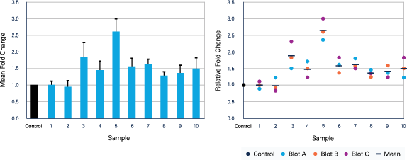
Using the normalized values, calculate the fold change (ratio of the experimental sample to the control) for each sample on replicate blot A (depicted in Figure 51).

BLOT A
Sample	Target, norm. intensity	Control, norm. intensity	Fold change
C	10,000	10,000	1.00
1	9,000	10,000	0.90
2	12,000	10,000	1.20
3	15,000	10,000	1.50
4	17,000	10,000	1.70
5	23,000	10,000	2.30
6	16,000	10,000	1.60
7	18,000	10,000	1.80
8	14,000	10,000	1.40
9	13,000	10,000	1.30
10	12,000	10,000	1.20

Figure 51. Fold change calculations: example data for Blot A. (left) In the blot diagram, C indicates the untreated control sample. Samples 1-10 received the experimental treatments. M indicates molecular weight marker. (right) Fold change was calculated for each band, using the normalized intensity values from Blot A. Each experimental sample is compared to the control, to generate a ratio. Example values are shown for illustration.

Repeat the fold change calculations with the normalized values from replicate blots B and C (depicted in Figure 52).

**Figure 52.** **Fold change calculations.** Example data are shown for Blots A, B, and C. *(top)* Strategy for calculating the fold change. *(bottom)* Fold change values for the three blots. In this illustration, samples 1-10 were loaded on replicate blots (Blots A, B, and C are technical replicates).

Using the fold change values from each replicate blot, calculate the mean fold change, overall % change, standard deviation, and coefficient of variation (CV) for all replicates (. Relative abundance of target protein, expressed as fold change and % change.).

Calculate the mean fold change of each replicate measurement.
Calculate the standard deviation of the fold change for each replicate measurement.

Calculate the coefficient of variation (CV) of the fold change for each replicate measurement.

**Table 3. Mean, % change, standard deviation, and CV calculations.** Example data are shown for analysis of samples 1-10 on Blots A, B, and C ( n = 3 technical replicates).
Sample	Blot A fold change	Blot B fold change	Blot C fold change	Mean fold change	% change	StDev	CV
C	1.00	1.00	1.00	1.00	0%	0.00	0%
1	0.90	1.00	1.10	1.00	0%	0.10	10%
2	1.20	0.90	0.80	0.97	-3%	0.21	22%
3	1.50	1.80	2.30	1.87	87%	0.40	22%
4	1.70	1.50	1.20	1.47	47%	0.25	17%
5	2.30	2.60	3.00	2.63	163%	0.35	13%
6	1.60	1.30	1.80	1.57	57%	0.25	16%
7	1.80	1.60	1.50	1.63	63%	0.15	9%
8	1.40	1.20	1.30	1.30	30%	0.10	8%
9	1.30	1.60	1.20	1.37	37%	0.21	15%
10	1.20	1.50	1.80	1.50	50%	0.30	20%

Plot the fold change in protein expression as a function of the treatment (Figure 53).
1. Some journals now prefer that small datasets be presented in scatterplot format, rather than the more typical bar graphs (9 - 10).
  - Scatterplots clearly show the spread and distribution of your data points, making it easier for peer reviewers and readers to fully understand your results.
  - Bar graphs are more suitable for large datasets. Many journals now discourage the use of error bars that indicate the standard error of measurement (SEM). Error bars that indicate the standard deviation of your measurements may be more appropriate (11, 12, 13).
  - Figure legends should clearly state what the error bars on the graph represent, and the value of n for the experiment. Sufficient detail should be provided to indicate if replicates are technical or biological.

**Figure 53.** **Bar graph and scatterplot of the fold change data in Table II.** *(left)* Mean fold change was plotted for each sample on a bar graph. Error bars indicate the standard deviation for each measurement (n = 3). The control is indicated by a black bar. *(right)* Fold change values from all blots were displayed as a scatterplot. The mean fold change for each sample is indicated by a horizontal line. The control sample is represented by a black dot. Technical replicates of samples 1-10 are shown (n = 3).

Data Interpretation

General guidelines are presented in this protocol. Appropriate replication and data interpretation are specific to each experiment, and beyond the scope of this protocol. Consult your local statistician for assistance.

Use the fold change and % change values for relative comparison of samples.
% change and CV can be used to evaluate the robustness of your QWB results, and determine if the magnitude of observed changes is large enough to be reliably distinguished from assay variability.
1. As described in Keys to Success, % change expresses the fold change as a percentage.
  - A positive number indicates an increase in relative abundance of target protein.
  - A negative number indicates decreased abundance.
2. The coefficient of variation (CV) describes the spread or variability of measured signals by expressing the standard deviation (SD) as a percent of the mean. Because CV is independent of the mean and has no unit of measure, it can be used to compare the variability of data sets and indicate the precision and reproducibility of an assay.
  - A low CV value indicates low signal variability and high precision of measurement.
  - A larger CV indicates greater variation in signal and reduced precision

On a Western blot, a change in band intensity is meaningful only if the magnitude of the % change substantially exceeds the CV (. CV and reported % change. The observed change in sample 2 (grey) is smaller than the CV of the measurement, and is not meaningful. In samples 8, 9, and 10 (orange), the reported change exceeds the CV by at least 2.5X. These changes are likely to be significant. Technical replicates of samples 1-10 are shown (n = 3).).

Generally speaking, the magnitude of the reported % change should be at least 2X greater than the CV of that measurement.

For example, to report a 20% difference between samples (0.8-fold or 1.2-fold change in band intensity), CV < 10% would be recommended for replicate samples. For a specific measurement, this threshold for the magnitude of change would correspond to the mean ± 2 SD.

In . CV and reported % change. The observed change in sample 2 (grey) is smaller than the CV of the measurement, and is not meaningful. In samples 8, 9, and 10 (orange), the reported change exceeds the CV by at least 2.5X. These changes are likely to be significant. Technical replicates of samples 1-10 are shown (n = 3)., the change observed in sample 2 is not meaningful (grey shading). A small change in target abundance was observed (-3%), but the CV of the measurement (22%) was larger than the effect.

Samples 8, 9, and 10 (orange shading) each showed a moderate increase in target abundance. In each case, the reported % change was considerably greater (>2.5X) than the CV of the fold-change measurement.

**Table 4. CV and reported % change.** The observed change in sample 2 (grey) is smaller than the CV of the measurement, and is not meaningful. In samples 8, 9, and 10 (orange), the reported change exceeds the CV by at least 2.5X. These changes are likely to be significant. Technical replicates of samples 1-10 are shown (n = 3).
Sample	Blot A fold change	Blot B fold change	Blot C fold change	Mean fold change	% Change	StDev	CV
C	1.00	1.00	1.00	1.00	0%	0.00	0%
1	0.90	1.00	1.10	1.00	0%	0.10	10%
2	1.20	0.90	0.80	0.97	-3%	0.21	22%
3	1.50	1.80	2.30	1.87	87%	0.40	22%
4	1.70	1.50	1.20	1.47	47%	0.25	17%
5	2.30	2.60	3.00	2.63	163%	0.35	13%
6	1.60	1.30	1.80	1.57	57%	0.25	16%
7	1.80	1.60	1.50	1.63	63%	0.15	9%
8	1.40	1.20	1.30	1.30	30%	0.10	8%
9	1.30	1.60	1.20	1.37	37%	0.21	15%
10	1.20	1.50	1.80	1.50	50%	0.30	20%

Faint bands or subtle changes in band intensity are more difficult to detect reliably. In these situations, QWB analysis requires more extensive replication and a lower CV.

Technical replicates: If the CV of your technical replicates is high, you may need to identify and reduce sources of error in your protocol to increase the precision of your assay. Technical replicates help you characterize the variability of your assay, so you can determine if the experimental response is reliable and meaningful.
Biological replicates: Interpret your technical replication data in the context of your biological replicates. A strong experimental response may be easily demonstrated, even with substantial technical variation. However, a weak or variable response may be very difficult to discriminate from the assay noise, and may require more extensive technical replication (1).

These are general guidelines only. Replication needs and data interpretation are specific to your experiment, and you may wish to consult a statistician.

References

1. Naegle K, Gough NR, Yaffe MB. Criteria for biological reproducibility: what does “n” mean? Sci Signal. 8(371): fs7 (2015).

2. Blainey P, Krzywinski M, Altman N. Replication: quality is often more important than quantity. Nat Meth. 11(9): 879-80 (2014).

3. Vaux DL, Fidler F, Cumming G. Replicates and repeats – what is the difference and is it significant? EMBO reports 13(4): 291-96 (2012).

4. Aldridge GM, Podrebarac DM, Greenough WT, Weiler IJ. The use of total protein stains as loading controls: an alternative to high-abundance single protein controls in semi-quantitative immunoblotting. J Neurosci Meth. 172(2): 250-54 (2008).

5. McDonough AA, Veiras LC, Minas JN, Ralph DL. Considerations when quantitating protein abundance by immunoblot. Am J Physiol Cell Physiol. 308: C426-C433 (2015).

6. Bakkenist CJ, Czambel RK, Hershberger PA, Tawbi H, Beumer JH, Schmitz JC. A quasi-quantitative dual multiplexed immunoblot method to simultaneously analysis ATM and H2AX phosphorylation in human peripheral blood mononuclear cells. Oncoscience 2(5): 542-54 (2015).

7. Plant AL, Locascio LE, May WE, Gallagher PD. Improved reproducibility by assuring confidence in measurements in biomedical research. Nat Meth. 11(9): 895-98 (2014).

8. Janes KA. An analysis of critical factors for quantitative immunoblotting. Sci Signal 8(371): rs2 (2015).

9. Fosang AJ, Colbran RJ. Transparency is the key to quality. J Biol Chem. 290: 29692-94 (2015).

10. Editorial. Towards greater reproducibility for life-sciences research in Nature. Nature 546: 8 (2017).

11. Krzywinski M, Altman N. Error bars. Nat Meth. 10(10): 921-22 (2013).

12. Fay DS, Gerow K. A biologist’s guide to statistical thinking and analysis. WormBook, ed. The C. elegans Research Community, WormBook, doi/10.189/wormbook.1.159.1, http://www.wormbook.org (2013).

13. Nagele P. Misuse of standard error of the mean (SEM) when reporting variability of a sample. A critical evaluation of four anaesthesia journals. Br J Anaesth. 90: 514-16.